Timepass: Replicating Jazayeri and Shadlen's Ready Set Go task

(A hobby psychophysics project)

TLDR: Replicated Jazayeri & Shadlen 2010’s time perception task and results: Ready Set Go task

Thinking about Time

I love thinking about how we perceive time. In school, during biology period, I would wait for the second hand to hit 12, close my eyes, and start counting. I’d open it at different intervals to see how accurate my internal clock was. (This might explain why I didn’t know what a gene really was till embarrassingly recently.) I wasn’t very good, but the fact that we can even attempt to do this raises a lot of questions. How am I able to mentally count? What’s this little stopwatch inside my head doing? What even is time?

Beyond my thrilling solitary sport of blindfolded time counting, several human and animal behaviors require precise timing, like a drummer maintaining a tempo, a tennis player timing their shot, or a predator pouncing on their prey. A basic computation that is central to all such behavior is interval timing: measuring the time between two events.

Vierordt’s law from The Sense of Time

One of the first systematic studies of interval timing was reported by Karl Vierordt in his 18XX book called Der Zeitsinn nach Versuchen - The Sense of Time According to Experiments. I don’t have access to the original text, but here’s a description from a different paper:

“For his main experiments—most of them were done by Vierordt himself as an only participant—his assistant produced a time interval with two clicks, and Vierordt replicated this interval by clicking a third time so that the interval between the second and third clicks was perceived as having the same duration as the interval between the first and second clicks.”

This experiment led him to discover a peculiar trend in his behavior: Shorter durations tend to be overestimated, whereas longer durations tend to be underestimated. This is called Vierordt’s law, and has since been replicated by several other studies ¹. Notably one by Jazayeri and Shadlen, where they rechristened this task ‘Ready Set Go’ (reminiscent of an official’s call before a race).

When I heard of this, I thought: First, that’s neat, I wonder why that’s happening. Can this tell us anything about how the brain processes temporal information? Second, the experiment sounds easy to replicate by myself, and seems like a good starting point to design further experiments to study time perception.

So I coded up the “Ready Set Go” task and piloted the task with myself as the subject to try and confirm Vierordt’s law and replicate the other effects in Jazayeri and Shadlen’s paper (henceforth JazShad).

Interval Timing in Ready Set Go

JazShad’s task was similar to Vierordt’s, except that they used visual stimuli instead of using sounds. On each trial, the intervals between the first and the second stimulus were drawn from a distribution with a particular mean. Each subject was tested on three different ‘prior conditions’, i.e. three different, but overlapping, ranges of interval durations (short, intermediate, and long). By doing so, they could study how subjects combine two sources of information: First, the (noisy) measurement of the interval on each trial. Second, the ‘prior’ information about the range of all intervals they might encounter on a given day. If you’re interested in how they do this, please see the section on the JazShad Model.

There were three main behavioral results from the subjects doing JazShad’s RSG. The beauty of this paper is that you can see all three of these effects in this single plot:

Figure 2 from Jazayeri and Shadlen 2010

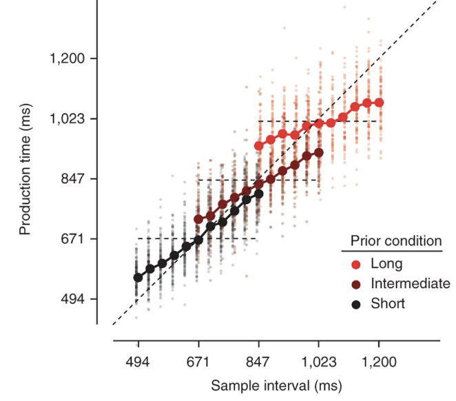
This plot shows the time durations reported by the subject on the y-axis (production times) against the actual sample intervals on the x-axis. The different colors correspond to the different prior conditions. The tiny dots are single trials and the large solid circles are the average across trials of a given sample interval and prior condition.

The three effects were: 1) Central tendency effect or Vierordt’s law: For each prior condition, the production times were systematically biased towards the mean value (horizontal dashed lines), with shorter durations being overestimated and longer durations being underestimated. 2) Scalar variability: Production times were more variable for the longer intervals. This one is admittedly a little harder to see in this plot, but the variance of the dots (single trials) for the longer duration trials are much more spread out than that for the shorter duration trials. 3) Bias scaling: Longer intervals tend to show greater bias to the mean duration. Production times for the short prior condition are much closer to the diagonal, i.e. much more accurate. Compare this to the long prior condition, where the production times for the extreme intervals tend to be farther away from the diagonal, implying that they were more biased towards the mean.

My time to shine: N=1 replication of RSG task

I set up my version of the ready set go task using JSPsych, a javascript library that lets you set up psychophsyics tasks that can run on a browser.

Each trial begins with the presentation of a red circle followed by an orange circle separated by some time duration. The subject must then wait for the same duration and press the [SPACE] button to make a green flash appear. Each trial is followed by a brief feedback period where the ‘error’, i.e. the difference between the reported and actual interval, is displayed.

Here’s how a single trial looks:

You can check out and run the task on yourself here: Ready Set Go Task.

At the end of the session, it’ll compile your behavior results and you can verify for yourself whether or not you adhered to Vierordt’s and Weber’s laws. If you would like to share your data with me so I can analyze it, please email it to me (mailto:adithyanarayan101@gmail.com). It will make me very happy.

Here’s my data:

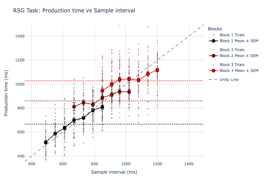
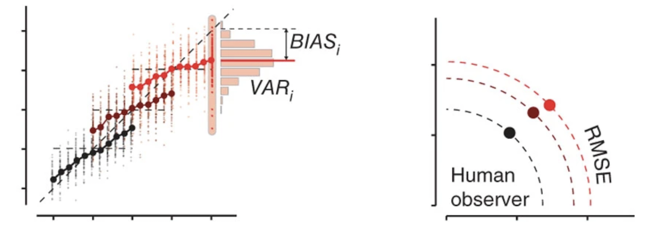
All three of the effects seen in the original JazShad paper seem to hold here as well. To visualize their results more clearly, they plot the bias (difference of production times from the actual interval) vs the variance (spread of production times) for each block.

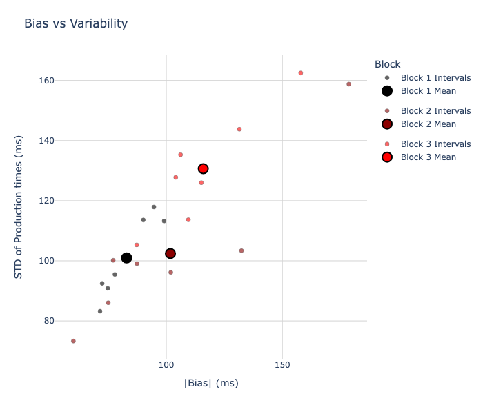
Below, you can see that: 1) the bias is non-zero (which means Vierordt’s law holds), 2) the variance is larger for the long block (scalar variability), and 3) the bias increases for the long block (bias scaling).

JazShad’s Variance vs Bias:

My data’s Variance vs Bias:

There were some differences as well, which I’ve documented here.

JazShad went on to formulate different bayesian ideal observer models to capture these behavioral trends and understand how humans combine prior and sensory information. I wrote a quick summary of their efforts for those interested: Modelling Time.

Next time

One of the most exciting and gratifying aspect of neuroscience is that it is the only subject where you get to be both the scientist and the subject of the study. I don’t just have to read a paper and know that Vierordt’s law is a thing, I’ve experienced it first hand. I’m happy that I’ve replicated the findings of Vierordt, JazShad, and many others ². This is where it gets fun. We can now ask a bunch of new questions that I’m not sure people have asked before.

A few questions that I’m thinking of:

• How do we maintain interval timing information in working memory?
• Does paying attention really slow down time?
• How much of the central tendency effect is due to processes that can be called ‘perception’ vs ‘cognitive’ vs ‘motor’?
  • I’m using these terms loosely, but it seems to me that I am not sure whether I am truly
    • perceiving the time intervals as being shorter or longer than they are (subjective sense of time changes),
    • or if I’m employing a decision strategy that maximizes my performance (I actually did perceive it as shorter, but I hedge my bets and report an interval closer to the mean)
    • or if I’ve formed some sort of motor bias, where it’s easier for me to learn to hit the button at roughly the same time after the second flash.

References

Temporal context calibrates interval timing - Jazayeri and Shadlen 2010

Extra stuff:

Discrepancies:

1) My ‘intermediate’ block data doesn’t quite fall right in between the short and the long. This could be due to limited data (they have 6 subjects doing at least 1500 trials each. I did a total of ~ 900. 2) They found that the bias towards the mean and the variability in production times were greater for the largest interval in each prior condition compared to the shortest, which is not the case in my data (could also be due to limited trial numbers): ![[Pasted image 20250809155758.png]]

Modelling Time!

JazShad set out to explain why human timing behavior follows Vierordt’s law. What they were seeking was a ‘normative’ model that fits human behavior: given certain assumptions and constraints, a normative model tells you what the optimal way is to solve a task.

The assumptions in the case of interval timing behavior are:

• The brain has to deal with internal noise. Neural responses are variable. The exact same stimulus elicits variable responses from the same neuron.
• This variability changes with the interval length. This is based on empirical evidence that longer intervals lead to more variable reproduction times. It’s termed ‘Scalar variability’ and a similar effect has been observed for various sensory variables (often called Weber’s law)
• The brain makes use of temporal regularities in the environment to guide behavior. Consider a musician trying to figure out when to play the next note. If he is unsure of when the last few notes were played, he can rely on his knowledge of the tempo of the song to infer when the next one should be.

JazShad formulated three different bayesian (see footnote if this word scares/annoys you) observer models to try and explain the data.

1) MLE: maximum likelihood estimation - we only care about the likelihood, i.e. the noisy measurement of the sample interval 2) MAP: maximum a posteriori - We combine the prior and likelihood to get the posterior, and then pick the mode of the posterior 3) BLS: we combine prior and likelihood and then pick the mean of the posterior.

If subjects were using the MLE algorithm, then we would expect the production times to not show any central tendency effects, since they are not using the prior information at all. Clearly, this isn’t the case. So we can discard this model. Both the MAP and the BLS models take into account the prior information as well as the likelihood information. Therefore, in both cases the production times will be biased towards the mean. However, comparing the performance of the two models, JazShad found that the BLS did a much better job explaining the trade-off between the bias and the variability in the production times.

By formulating multiple normative models that are based on different assumptions and comparing them to see which one matches human behavior, we can tell something about the kinds of constraints that the brain is working with. We can then go on to study the brain and verify how and if these algorithms are actually implemented in wetware. In true Marr-ian (footnote) fashion, Jazayeri did just that for interval timing behavior and published a series of brilliant papers [cite jaz neural]

1. Aren’t you wondering what Vierdort’s law has to do with management principles? Yeah, me neither. But someone wrote a rather misguided post about “how you can apply Vierordt’s Law to project management to achieve your project goals” , a really nifty piece of truth-bending. ↩

2. Vierordt’s law: a consequence of randomization? In lab behavioral tasks, it is common practice to test different trial types in a random order to prevent the subjects from building expectations based on recent history. This allows the experimenter to treat each trial as independent. This is obviously not the case in nature. In real life, things change in a continuous, and typically slow, manner. Glasauer and Shi 2021 makes an interesting case that Vierordt’s law might be a consequence of the unnatural experimental randomization protocol. They show that when subjects are tested on a similar experiment but with time intervals that vary slowly across trials, the central tendency effect is reduced. It’s a neat paper and a good reminder to carefully think about the consequences of experimental choices, even ones that the field cherishes and takes for granted. ↩